Graham’s Biggest Little Hexagon

Think of the following problem: What is the largest area of a Hexagon with diameter equal to 1?

As is the case with many questions similar to the one above, called polygonal isoperimetric problems, the first guess is the regular hexagon. For example, the largest area of a Hexagon with fixed perimeter is obtained for the regular hexagon. However, for the initial question, the regular hexagon is not the best one. Graham proved in his paper “The largest small hexagon” that there exists a better competitor and he showed precisely which hexagon is optimal. More details on the history of the problem and more references can be found in Graham’s paper, the Wikipedia page or the Mathworld page.

I recently wanted to use this hexagon in some computations and I was surprised I could not find explicitly the coordinates of such a hexagon. The paper “Isodiametric Problems for Polygons” by Mossinghoff was as close as possible to what I was looking for, although the construction is not explicit. Therefore, below I present a strategy to find what is the optimal hexagon and I will give a precise (although approximate) variant for the coordinates of Graham’s hexagon.

Weitzenböck’s inequality – graphical proof

As discussed in a previous post for any triangle we have the inequality 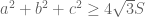where are the side lengths and is the area. Various proofs exist, however, there is a very beautiful visual one due to  Claudi Alsina, Roger B. Nelsen: Geometric Proofs of the Weitzenböck and Hadwiger–Finsler Inequalities. Mathematics Magazine, Vol. 81, No. 3 (Jun., 2008), pp. 216–219

Consider first the case where all angles are smaller than 120 degrees. Then construct the Fermat point (or Torricelli point) which corresponds to the minimizer of the sum . From the optimality condition, the angles at must be equal. Construct now equilateral triangles outside the triangle and note that triangles , can all be put three times inside the corresponding equilateral triangle. Writing down everything, together with the formula for the area of an equilateral triangle gives you the result!

The quantitative form, namely the Hadwiger-Finsler inequality, can also be obtained from this construction. But more on this in some other post. For now, just take a look at the picture below and try to understand this very nice geometric proof!

Proof of the Isoperimetric Inequality 3

I will present here a third proof for the planar Isoperimetric Inequality, using some simple notions of differential curves. For this suppose that the simple closed plane curve has length and encloses area . Then

and equality holds if and only if is a circle.

Proof of the isoperimetric inequality 2

I will continue the series of proofs for the isoperimetric inequality in the two dimensional case, i.e. if a simple closed curve (which we suppose for simplicity that it consists of piecewise curves) of length encloses an area then and the equality is attained only if is the boundary of a circle.

Proof of the Isoperimetric Inequality

The Isoperimetric inequality gives a bound for the area in terms of the perimeter of a set. It says that the greatest area that can be enclosed by a curve which has length is maximal when the curve is the boundary of a circle, or equivalently the minimum of the perimeter of a curve which encloses a set of area is attained again for the circle. In two dimension the inequality says that where is the perimeter and is the area (Lebesgue measure) of a plane region .

Region which can sustain the Largest Sandpile

Among all plane regions which are open and simply connected and without holes of given area the circle can support the largest sandpile.

Leavitt and Ungar – Circle supports the largest sandpile.

Existence Result for the Isoperimetric Problems

The tricky part is how to define the perimeter of a Lebesgue measurable set with finite perimeter. This can be done considering the space of bounded variation functions, denoted . By definition we have for an open set that .  Here we denoted by the space of continuously differentiable functions with compact support in . Because of the density of the space of infinitely differentiable functions with compact support in in the space , we could have replaced by in the above definition. You could take a look at this blog post for a detailed description of or at the Wikipedia page.

We say that a set of finite Lebesgue measure is a set of finite perimeter in if its characteristic function belongs to . This means that the distributional gradient is a vector valued measure with finite total variation. The total variation is called the perimeter of .

In the same way we can define the perimeter of a Lebesgue measurable set relative to an open set . We say that is a set of finite perimeter relative to if the characteristic function belongs to the space .