Is the Earth flat?

Consider the following experiment: the pairwise distances between four cities on Earth are given. Can you answer the following questions:

1) Can these distances be realized in a flat Earth?

2) Assuming the Earth is spherical and distances are measured along geodesics, can you determine the radius?

The test case was inspired from the following note. The initial test case involves the cities: Seattle, Boston, Los Angeles and Miami. A second test case is provided below.

You can use the Python code to create new test cases of your own. 

Explicit Euler Method – practical aspects

In a previous post I presented the classical Euler methods and how they apply to the simple pendulum equation. Let me now be a little more explicit regarding the coding part. I will present a Python code and give you some main ideas, important from my point of view, regarding the implementation. Here is a summary of these ideas

• Use numpy in Python. When performing numerical simulations related to ODEs it is recommended to work in floating point precision. This will give you accurate enough results (at least for usual academical examples) and will produce a more efficient code.
• Structure the code using functions. The code for the Explicit Euler method should be easily adaptable to other problems, by changing the function defining the ODE (like shown in this post)
• Any numerically implemented method for solving ODEs should be tested on a simple example where the analytical solution is known. In particular, the convergence order of the method can be identified and should coincide with the theoretical prediction. This can easily help debug implementation errors for more complex methods.
• When the ODE comes from an isolated system where there is an invariant (like the energy for the pendulum), the numerical preservation of this invariant should be tested. Errors might be seen, but they should be quantifiable in terms of the step size and the order of the method. Aberrant results here could indicate the presence of a bug.

Simple Pendulum – Euler methods

Given , Lipschitz in the second variable, consider the ODE

In most cases where equation (1) models some real world phenomena, the solutions are not explicit. Therefore, numerical methods are developed in order to solve such problems.

The simple pedulum

In physics the simple pendulum is a punctual mass fixed at the extremity of a wire without mass and in-extensible (or rigid), which oscillates under the effect of gravity. It is straightforward to see that if the point of attachment of the wire is fixed, then the resulting dynamical system can be uniquely determined knowing the inclination of the wire with the vertical and the parameters of the system (mass, length of wire, gravitational acceleration). The easiest way of deriving the equation of movement for the pendulum (supposing there is no friction) is to write the total energy of the system. The angular speed of the pendulum being we find that the speed of the point mass is . This shows that the kinetic energy of the mass is . The potential energy due to the gravitational force is , assuming that corresponds to zero height. Therefore, the total energy is given by

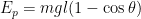
Supposing the system is isolated and no energy is lost due to friction we have that the derivative of the energy with respect to time is zero:

Checking the gradient and Hessian implementation using finite differences

Solving a numerical optimization problem depends not only on the optimization algorithm you use, but also on the fact that you implemented correctly the gradient and, eventually, the Hessian matrix associated to the function you want to optimize. The correct implementation of the partial derivatives is not always a trivial calculus question, where you have an analytic formula for your function and you just need to take care when performing the computations. However, even the best students can make a typing error, put a wrong sign somewhere, miss a factor, etc, and in that case the optimization algorithm simply doesn’t work as expected.

Things get even more complicated when the computation of the gradient (and Hessian) goes through some PDE model, multiplying the places in your code where an error might hide. For example in some parametric shape optimization problem, one has a parametric description of the shape and the gradient of the function to be optimized is obtained by putting in the associated shape derivative formula a perturbation field associated to the variation in the corresponding parameter.

Gradient algorithm with optimal step: Quadratic Case: theory

In a previous post I looked at the theory behind the convergence of the gradient descent algorithm with fixed step for a quadratic function. In this post I will treat a similar topic, namely the gradient descent algorithm with optimal step for the case of a quadratic function. Let us consider again defined by

the classical quadratic function, where is symmetric positive definite and is an arbitrary vector. The gradient descent algorithm with optimal step has the form

where the descent step is chosen such that

is minimal.

Gradient algorithm: Quadratic Case: theory

Everyone who did a little bit of numerical optimization knows the principle gradient descent algorithm. This is the simplest gradient based algorithm: given the current iterate, advance in the opposite direction of the gradient with a given step

It is straightforward to see that if is small enough, and is at least then

This means that there exists a small enough for which .

Recurrences converging to the wrong limit in finite precision

Consider the following recurrence:

a) Study this recurrence theoretically: prove that the sequence converges and find its limit.

b) Implement the recurrence using the programming language of your choice and see what is the limit obtained by numerical investigation. Interpret the results!

Gradient Descent converging to a Saddle Point

Gradient descent (GD) algorithms search numerically for minimizers of functions . Once an initialization is chosen the algorithm is defined by

where is a descent step, often found using a particular line-search procedure. It is widely known that GD algorithms converge to critical points under very mild hypotheses on the function and on the line-search procedure. Moreover, GD algorithms almost always converge to local minimizers (convergence to the global minimizer is hard to guarantee, except in the convex case).

However, the “almost always” part from the above sentence is in itself interesting. It turns out that the choice of the initialization may lead the algorithm to get stuck in a Saddle Point, i.e. a critical point where the Hessian matrix has both positive and negative eigenvalues. The way to imagine such examples is to note that at such a Saddle Point there are directions for which is minimized and directions for which is maximized. If the gradient only contains information in the direction where is minimized, the algorithm will stop there. However, the set of initializations for which GD will get stuck in a Saddle Point is very small and considering slightly perturbed initializations might solve the problem.

To better illustrate this phenomenon, let’s look at a two dimensional example:

It can be seen immediately that this function has critical points at and that is a saddle point, while the other two are local minima. A graph of this function around the origin is shown below

Note that looking only along the line the saddle point is a minimizer. Therefore, choosing an initialization on this line will make the GD algorithm be stuck in the Saddle Point . Below you can see an example for the initialization , and the trajectory of the GD algorithm is illustrated. Considering only a slight perturbation allows the GD algorithm to escape the saddle point and to converge to a local minimizer.

 

One simple way to prevent GD algorithms being stuck in a saddle point is to consider randomized initializations so that you avoid any bias you might have regarding the objective function.

On Heron’s algorithm – approximating the square root

Heron’s algorithm computes an approximation of the square root of a positive real number using the iteration

1. Show that the recurrence defined above is Newton’s algorithm applied for finding a zero of the function . Show that the sequence converges to when is close enough to . What is the order of convergence of the sequence?In the following we consider the following error measure:

   

   This choice simplifies the computations and is an estimation of half the relative error when .

2. Show that the sequence verifies

   

   Deduce an explicit formula for in terms of . Show that the sequence converges to for every choice of the initial condition .

3. Show that for every there exists an integer such that . Write a modified Heron algorithm which reduces the computation of the square root of to the computation of the square root of a real number .The choice of the initialization determines and has an influence on the speed of convergence. In the following we restrict ourselves to the case and we look at the choice of the initial condition. We will suppose that the initial condition depends on and we will consider the following cases: , a constant function and , a polynomial of degree in . In every case we will try to minimize for .
4. Show that if then is minimal for . Find the explicit value of . (Hint: You could represent graphically the function .)
5. Suppose that is a polynomial of degree in . We want to find the coefficients and which minimize with .
   (a) Prove that the maximum of is found for .
   (b) Show that in order to minimize it is necessary that and that .
   (c) Conclude that the and which minimize are . Find an exact expression for .
6. For compare the number of iterations necessary to arrive at a demanded precision ( for the two initializations studied: and with . Comment on the interest of using the initialization of degree compared to the constant initialization
7. Evaluate the number of operations used for the two cases and conclude which of the two approaches is more advantageous.
8. Try to find the initialization of second degree which is optimal and perform a similar investigation to see if from the point of view of the number of operations this choice is well adapted or not.

Condition number of a matrix

Let be a real matrix which is invertible. For a vector we solve the system

The condition number of a matrix gives an idea on the behavior of the solutions with respect to perturbations of the vector . Given a perturbation , consider the solution of the associated system:

1. If , show that

where

This quantity is the condition number of . Note that the condition number depends on the chosen norm.

2. Show that if is invertible and symmetric and we consider the Euclidean norm, then

where is the condition number for the norm . Hint: Use the fact that is diagonalizable in an orthonormal basis.

3. Consider the following example (attributed to H. Rutishauser) :

Compute the determinant of and the inverse of . You can use numerical tools like “numpy.linalg.inv” and “numpy.linalg.det”. Solve the systems and using either the inverse found previously or “numpy.linalg.solve”. Explain the behavior obtained and give a lower bound for the condition number of the matrix . Compute the condition number of using the following methods

• compute the eigenvalues of with “numpy.linalg.eig” and use the previous point
• use “numpy.linalg.cond”

Conclude that the lower bound found previously was not so far from the condition number. Try to find other examples of and which can get you arbitrarily close to the condition number.

Integrating an oscillatory function

Consider the function extended in zero with . The objective of this exercise is to prove that the integral exists and to give a numerical approximation of . A graphical representation of is shown below:

1. Use your favorite numerical tool (for example \texttt{scipy.integrate}) in order to evaluate directly the integral on . Explain the eventual error messages and comment on the eventual error messages obtained.

2. Consider the decreasing sequence of zeros of . Obtain the integral of like a series of integrals of on the intervals . Use again your favorite numerical tool (e.g. \texttt{scipy.integrate}) for each of the previous intervals for . Find a good stopping criterion which says you have found a good approximation of . How can you accelerate the convergence. What other choice do you have for the choice of the sequence ?

3. Show that

Evaluate this expression with the aid of a numerical software and compare the precision to the result obtained at the previous points. Explain the eventual gain of precision compared to point 1. 4. The function integral cosine is defined by

Prove that . Use a numerical tool which allows you to obtain to machine precision.

Remark: The precise evaluation of can be found using the following series representation of on :

where is the Euler-Mascheroni constant. 5. Consider the function defined by .

Show that the integral corresponds to the imaginary part of on the path , . Consider the alternative path , .

Prove that is bounded in the region . Deduce using Cauchy’s theorem that

Prove that on the new path the function does not oscillate. Moreover, as on the converges exponentially to zero.

Use a numerical tool (e.g. \texttt{scipy.integrate}) to compute the integral of on the path . Recall that:

Compare the result to the ones obtained before and conclude why the numerical software manages to approximate correctly the integral of on the path .

What can go wrong with numerics

I recently watched the video Validated Numerics by Warwick Tucker. This video is an introduction to interval arithmetic, which is a rigorous way of doing numerics with nice applications. In the first part of the video, however, he starts by showing some examples where the numerics can go wrong.

First, in order to understand why computations done by a machine can be wrong, you need to know how the computer looks at numbers. Since the computer has a finite amount of memory, it will never store exact representations. Irrational numbers with infinitely many digits repeating without any pattern whatsoever are clearly not representable. Even rational numbers, which are the ratios of two integers may be costly to represent if the integers involved are quite large. When working with simulations one often manipulates not one variable but vectors and matrices with millions of variables. Therefore it is necessary to bound the memory allocated to each one of these variables. This is why the floating point arithmetic was introduced.

A floating point number (in some basis, binary for the computer, decimal for the usual representation) is composed of a real number m called the mantissa and an exponent e. The catch is that the mantissa will store only finitely many digits and usually it is normalized, i.e. there are no zeros after the decimal point. For example:

• 1.01011 is a valid mantissa with 5 binary digits (the leading 1 is not counted)
• 0.00101 is not a normalized mantissa since there are zeros after the decimal point
• 1011.01 is not a normalized mantissa since there are more then one digits before the decimal point

The mantissa alone, in binary representation, will only represent numbers between 1 and 2. However, one can reach more numbers using a multiplication with a power of two, contained in the exponent. Therefore, the computer knows a number by its finite precision mantissa and its exponent. The sign of the number can also be included in one bit. I will not try to make an exhaustive lecture on floating point representations: you should check other references for more information.

Using this floating point representation, the problem of memory is solved, but the thing is that operations using floating point numbers are not exact. In order to make an addition the computer needs to shift the decimal point so that the two numbers have the decimal point at the same place. The problem is that every time this is done, information is lost at the other end of the mantissa.

The following example is shown in the book “Validated Numerics” and is due to Rumpf (the creator of Intlab, an interval arithmetic for Matlab). Consider the function

Then, depending on the size of the floating point representation or on the convention made when performing the rounding the evaluation of gives different results. The idea is that the two terms and evaluated at the corresponding point give rougly the same digit number. Their exact sum is which coupled with the last term should give .

However, when adding those two huge numbers multiple things may happen:

• the computer sees that they are roughly the same so it supposes that their difference is zero
• the computer makes some random operation after the 21th digit in 64 bits (where we roughly have 16 significant digits of precision)

In the end, the result shown is not correct, unless we work with multiple precision arithmetics.

This should not discourage us in using numerical computations, which are useful in many practical application. On the other hand we should be aware that when doing computations in floating point representation results are only approximate. Particular care should be made when subtracting two numbers which are close but which are not exactly represented using the floating point system.

 

FreeFem++ Tutorial – Part 1

First of all, FreeFem is a numerical computing software which allows a fast and automatized treatment of a variety of problems related to partial differential equations. Its name, FreeFem, speaks for itself: it is free and it uses the finite element method. Here are a few reasons for which you may choose to use FreeFem for a certain task:

1. It allows the user to easily define 2D (and 3D) geometries and it does all the work regarding the construction of meshes on these domains.
2. The problems you want to solve can be easily written in the program once we know their weak forms.
3. Once we have variables defined on meshes or solutions to some PDE, we can easily compute all sorts of quantities like integral energies, etc.

Before showing a first example, you need to install FreeFem. If you are not familiar with command line work or you just want to get to work, like me, you can install the visual version of FreeFem which is available here. Of course, you can find example programs in the FreeFem manual or by making a brief search on the internet.

I’ll present some basic stuff, which will allow us in the end to solve the Laplace equation in a circular domain. Once we have the structure of the program, it is possible to change the shape of the domain in no time.

Even small errors can be fatal

Machines and computers represent numbers as sequences of zeros and ones called bits. The reason for doing this is the simplicity of constructing circuits dealing with two states. This fact coupled with limited memory capacities means that from the start we cannot represent all numbers in machine code. It is true that we can get as close as we want to any number with great memory cost when precision is important, but in fact we always use a fixed precision. In applications this precision is fixed to a number of bits (16, 32, 64) which correspond to significant digits in computations. Doing math operations to numbers represented on bits may lead to loss of information. Consider the following addition using significant digits:

notice that using only the first significant digits we have made an error of . This may seem small, but if we do not pay attention and we let errors of this kind accumulate we may have a final error which is unacceptable. This is what happened in the case of the Patriot missile case which I’ll discuss briefly below.

Solving Poisson’s equation on a general shape using finite differences

One of the questions I received in the comments to my old post on solving Laplace equation (in fact this is Poisson’s equation) using finite differences was how to apply this procedure on arbitrary domains. It is not possible to use this method directly on general domains. The main problem is the fact that, unlike in the case of a square of rectangular domain, when we have a general shape, the boudary can have any orientation, not only the orientation of the coordinate axes. One way to avoid approach this problem would be using the Finite Element Method. Briefly, you discretize the boundary, you consider a triangulation of the domain with respect to this discretization, then you consider functions which are polynomial and have support in a few number of triangles. Thus the problem is reduced to a finite dimensional one, which can be written as a matrix problem. The implementation is not straightforward, since you need to conceive algorithms for doing the discretization and triangulation of your domain.

One other approach is to consider a rectangle which contains the shape and add a penalization on the exterior of your domain . The problem to solve becomes something like:

where is defined by

Note that doing this we do not need to impose the boundary condition on . This is already imposed by , and the fact that is forced to be zero outside .

Simple optimization problem regarding distances

Given points in the plane we can study the problem

For the solution is known and for a triangle which has an angle less than is the Toricelli (or Fermat) point, which lies at the intersection of the circumcircles of the equilateral triangles built outside the triangle having the sides of the triangle as support.

For , if we have a convex quadrilateral, then a simple triangle inequality argument proves that the optimal position for is the intersection of the diagonals.

In general, we cannot precisely say what is the position of the solution. Providing a numerical algorithm which computes the optimal position of is not a hard task, and I will do that in the end of this post.

 

Numerical method – minimizing eigenvalues on polygons

I will present here an algorithm to find numerically the polygon with sides which minimizes the -th eigenvalue of the Dirichlet Laplacian with a volume constraint.

The first question is: how do we calculate the eigenvalues of a polygon? I adapted a variant of the method of fundamental solutions (see the general 2D case here) for the polygonal case. The method of fundamental solutions consists in finding a function which already satisfies the equation on the whole plane, and see that it is zero on the boundary of the desired shape. We choose the fundamental solutions as being the radial functions where are some well chosen source points and . We search our solution as a linear combination of the functions , so we will have to solve a system of the form

in order to find the desired eigenfunction. Since we cannot solve numerically this system for every we choose a discretization on the boundary of and we arrive at a system of equations like:

and this system has a nontrivial solution if and only if the matrix is singular. The values for which is singular are exactly the square roots of the eigenvalues of our domain .

Best approximation of a certain square root

Let be a real number such that the inequality

holds for an infinity of pairs of natural numbers. Prove that .

Distance from a point to an ellipsoid

Here I will discuss the problem of finding the point which realizes the minimal distance from a given to an ellipsoid. First I will look at the theoretical properties which will lead us to and then I will present a numerical algorithm to find the nearest point.

This problem is interesting in itself, but has some other applications. Sometimes in optimization problems we need to impose a quadratic constraint, so after a gradient descent we always project the result on the constraint which is an ellipsoid.

Let’s begin with the problem, which can be formulated in a general way like this: we are given , and a matrix , positive semidefinite, which gives an ellipsoid . Without loss of generality assume that is diagonal (if not, we diagonalize it using an orthogonal matrix and work in a new coordinate system). The problem becomes

(note that the square is not important here, but simplifies the computations later)