Best linear interpolation constant on a triangle
Given a triangle 


When dealing with finite element estimations it is a natural question to try and bound the difference of the gradients in 


where 
Let me name a few papers where such results are discussed:
- Estimation of interpolation error constants for the P0 and P1 triangular finite elements by Fumio Kikuchi and Xuefeng Liu: https://doi.org/10.1016/j.cma.2006.10.029 In this paper, explicit formulas for
- For a fixed triangle
- Kobayashi proposes multiple explicit formulas for the constant C in https://am2015.math.cas.cz/proceedings/contributions/kobayashi.pdf The proofs are not complete, but they are verified for a large class of triangles through discrete eigenvalue problems. Indeed, using a triangulation of
with the Morley finite elements gives an explicit upper bound for the constant.
Iterative algorithms – Convergence rates
In optimization and any other iterative numerical algorithms, we are interested in having convergence estimates for all algorithms. We are not only interested in showing that the error goes to 
Generally, there are two points of view for convergence: convergence in terms of 


To fix the ideas, denote 


We have the following standard classification:
- linear convergence: there exists
such that
the constant
, so in particular
.
- sublinear convergence:
- superlinear convergence:
with any positive convergence ratio
- {convergence of order
}: there exists
such that for
large enough
is called the order of convergence
has a special name: quadratic convergence


To underline the significant difference between linear and superlinear convergence consider the following examples: Let 
converges linearly to zero, but not superlinearly
converges superlinearly to zero, but not quadratically
converges to zero quadratically
Quadratic convergence is much faster than linear convergence.
Among optimization algorithm, the simpler ones are usually linearly convergent (bracketing algorithms: trisection, Golden search, Bisection algorithm, gradient descent). Algorithms involving higher order information or approximation are generally superlinear (Secant method, Newton, BFGS or LBFGS in higher dimensions etc.).
There is a huge difference between linear convergence and super-linear convergence. If a faster algorithm is available using it is surely useful!
Golden search algorithm – efficient 1D gradient free optimization
Bracketing algorithms for minimizing one dimensional unimodal functions have the form:
- Suppose
is an interval containing the minimizer
- Pick
in
- If
then choose
- If
then choose
- Stop the process when
![{[a_{n+1},b_{n+1}] = [a_n,x^+]}](https://s0.wp.com/latex.php?latex=%7B%5Ba_%7Bn%2B1%7D%2Cb_%7Bn%2B1%7D%5D+%3D+%5Ba_n%2Cx%5E%2B%5D%7D&bg=ffffff&fg=000000&s=0&c=20201002)
![{[a_{n+1},b_{n+1}] = [x^-,b_n]}](https://s0.wp.com/latex.php?latex=%7B%5Ba_%7Bn%2B1%7D%2Cb_%7Bn%2B1%7D%5D+%3D+%5Bx%5E-%2Cb_n%5D%7D&bg=ffffff&fg=000000&s=0&c=20201002)
The simplest algorithm corresponds to choosing 

Optimizing a 1D function – trisection algorithm
Optimization problems take the classical form

Not all such problems have explicit solution, therefore numerical algorithms may help approximate potential solutions.
Numerical algorithms generally produce a sequence which approximates the minimizer. Information regarding function values and its derivatives are used to generate such an approximation.
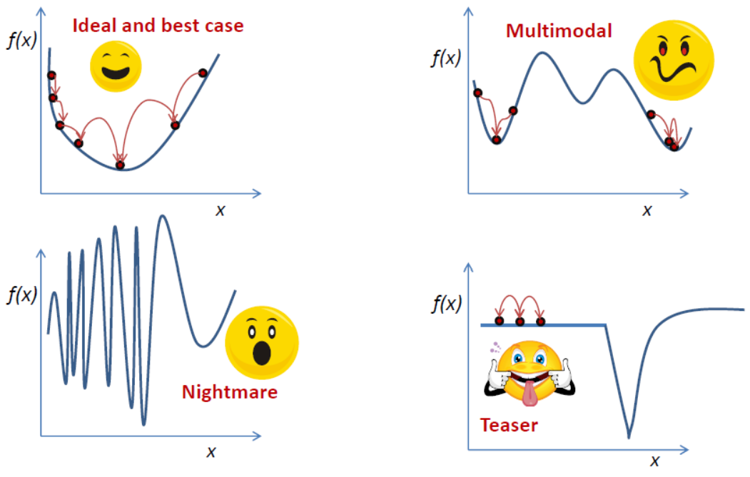
The easiest context is one dimensional optimization. The basic intuition regarding optimization algorithms starts by understanding the 1D case. Not all problems are easy to handle for a numerical optimization algorithm. Take a look at the picture below:
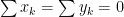
An inequality involving complex numbers
Consider 

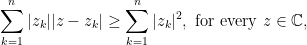
if and only if 
Proposed by Dan Stefan Marinescu in the Romanian Mathematical Gazette
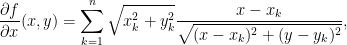
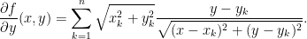
Solution: For someone familiar with optimality conditions in multi-variable calculus this is straightforward. Notice that
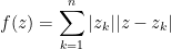
is a convex function (linear combination of distances in the plane). The inequality is equivalent to 
For a convex, differentiable function global minimality is equivalent to verifying first order optimality conditions. Denoting 


If 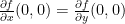
Since this problem was proposed for 10th grade, let’s use some simpler arguments to arrive to a proof. Denote by 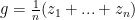
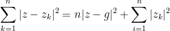
Thus 

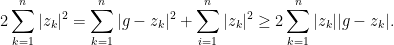
If the inequality in the statement of the problem holds, the above relation becomes an equality and 


Conversely, if 

Romanian Regional Olympiad 2024 – 10th grade
Problem 1. Let 


Problem 2. Consider 


a) Prove that if the triangle 

b) Show that if there exist three distinct points 
Problem 3. Let 


Problem 4. Let 


for every 

Hints:
Problem 1: study the monotonicity of the function 

Problem 2: Recall the identity 


Problem 3: Denote 


Problem 4. Take 


Putnam 2023 A1-A3
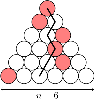
A1. For a positive integer 

Hints: Observe that
Differentiate again and observe that

It is straightforward now to evaluate 
A2. Let 


Hints: Denote 


It follows that 


A3. Determine the smallest positive real number 


- (a)
,
- (b)
,
- (c)
for all
- (d)
for all
- (e)
.
Hints: Of course, an example of functions 


Assuming that ![{[0,r]}](https://s0.wp.com/latex.php?latex=%7B%5B0%2Cr%5D%7D&bg=ffffff&fg=000000&s=0&c=20201002)

where the last inequality follows from 
Therefore 
Therefore we have 
The initial conditions show that 
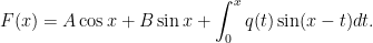
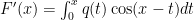
![\displaystyle F(x) = \int_0^x q(t)\sin(x-t)dt, x\in [0,r]](https://s0.wp.com/latex.php?latex=%5Cdisplaystyle+F%28x%29+%3D+%5Cint_0%5Ex+q%28t%29%5Csin%28x-t%29dt%2C+x%5Cin+%5B0%2Cr%5D&bg=ffffff&fg=000000&s=0&c=20201002)
and since 

![\displaystyle f(x)-f(0)\cos x\geq 0, x \in [0,r].](https://s0.wp.com/latex.php?latex=%5Cdisplaystyle+f%28x%29-f%280%29%5Ccos+x%5Cgeq+0%2C+x+%5Cin+%5B0%2Cr%5D.&bg=ffffff&fg=000000&s=0&c=20201002)
Thus the smallest 
Algebraic proof of the Finsler-Hadwiger inequality
Weitzenbock’s inequality states that if 
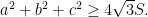
A strengthening of this result due to Finsler and Hadwiger states

A variety of proofs rely on various trigonometric or geometric arguments. Below you can find a purely algebraic argument based on the classical characterization: 


Replacing

and

On the other hand the area given by Heron’s formula is
Thus, Weitzenbock’s inequality is equivalent to

and the Finsler-Hadwiger inequality is equivalent to
This inequality follows at once, since squaring both sides gives
which is a well known consequence of

Equality holds, of course, if and only if 
A proof of the Hadwiger Finsler inequality
The Hadwiger-Finsler inequality states that if

This was discussed previously on the blog. This post shows a translation of the original paper by Hadwiger and Finsler and this post shows a surprising geometrical proof.
Various proofs of the inequality are known. However, since an equality always beats an inequality, let us prove the identity

It is immediate to see that Jensen’s inequality applied to the tangent function, which is convex on ![{[0,\pi/2]}](https://s0.wp.com/latex.php?latex=%7B%5B0%2C%5Cpi%2F2%5D%7D&bg=ffffff&fg=000000&s=0&c=20201002)

Replacing the usual formula 
Summing these identities for the three angles 
Is the Earth flat?
Consider the following experiment: the pairwise distances between four cities on Earth are given. Can you answer the following questions:
1) Can these distances be realized in a flat Earth?
2) Assuming the Earth is spherical and distances are measured along geodesics, can you determine the radius?
The test case was inspired from the following note. The initial test case involves the cities: Seattle, Boston, Los Angeles and Miami. A second test case is provided below.

You can use the Python code to create new test cases of your own.
Read more…Area of a spherical triangle
A spherical triangle is obtained by joining three points 


where 
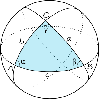
Proof: Draw the great circles associated to 


The image was taken from here.
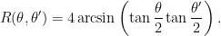
Area of a spherical rectangle
A spherical rectangle is a spherical geodesic quadrilateral whose vertices 

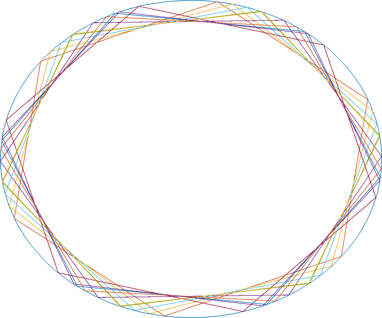
Maximal area polygons contained in disk/ellipse
Consider the unit disk 

Deduce that the maximal area
This was inspired by the following MathOverflow question.
Solution: Obviously, a maximal area polygon will be convex, otherwise take the convex hull.
First, observe that an 


Moreover, any maximal area polygon must contain the center of
Such a polygon is completely characterized (up to a permutation of its sides) by the lengths of its sides, or equivalently, the angles at the center of ![{\theta_1,...,\theta_n\in [0,\pi]}](https://s0.wp.com/latex.php?latex=%7B%5Ctheta_1%2C...%2C%5Ctheta_n%5Cin+%5B0%2C%5Cpi%5D%7D&bg=ffffff&fg=000000&s=0&c=20201002)
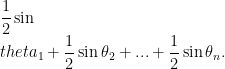
Since 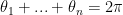
![{[0,\pi]}](https://s0.wp.com/latex.php?latex=%7B%5B0%2C%5Cpi%5D%7D&bg=ffffff&fg=000000&s=0&c=20201002)
Any ellipse is an image of the disk through an affine transformation. Since affine transformations preserve area ratios, any image of a in inscribed regular
IMO 2023 Problem 2
Problem 2. Let 


Prove that the line tangent to 
Solution: Let us first do some angle chasing. Since 


Denote by 


Let us denote 


Moreover, 
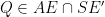


On the other hand, 


There are quite a few inscribed hexagon where Pascal’s theorem could be applied. Moreover, to reach the conclusion of the problem it would be enough to prove that 


IMO 2023 Problem 4
Problem 4. Let 


IMO 2023 Problem 1
Problem 1. Determine all composite integers 


Problems of the International Mathematical Olympiad 2023
Problem 1. Determine all composite integers
Problem 2. Let
Problem 3. For each integer 


for every integer 
Problem 4. Let
is an integer for every
Problem 5. Let 


In terms of
Problem 6. Let 


Let 


(Note: a scalene triangle is one where no two sides have equal length.)
Source: imo-official.org, AOPS forums
Polygon with an odd number of sides
Let 


Alternative reformulation: Let 

Romanian Team Selection test 2007
Read more…A series involving a multiplicative function
Let 


Prove that

I posted this problem quite a while back. Here is a solution I found recently.
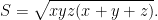
Read more…Maximize the circumradius of a unit diameter simplex
Given a simplex in dimension 
Consider 


An immediate upper bound, which is tight can be obtained from the identity 


Beni Bogoşel

Click to see my CV
Today’s Visitors

Click for more info
