Iterative algorithms – Convergence rates

In optimization and any other iterative numerical algorithms, we are interested in having convergence estimates for all algorithms. We are not only interested in showing that the error goes to , although that is essential, but also at what speed the error goes to . An algorithm which converges quicker is a better choice in all cases!

Generally, there are two points of view for convergence: convergence in terms of where is the number of iterations or having a comparison between the error at iteration and the error at the iteration . I will take the latter point of view below.

To fix the ideas, denote the error estimate for , where is the current iterate and is the solution to the problem.

We have the following standard classification:

• linear convergence: there exists such that
  the constant is called the convergence ratio  it is easy to show that , so in particular .
• sublinear convergence:  but is not linearly converging
• superlinear convergence:  with any positive convergence ratio
   sufficient condition:
• {convergence of order }: there exists such that for large enough
  is called the order of convergence 
  the case has a special name: quadratic convergence

To underline the significant difference between linear and superlinear convergence consider the following examples: Let . Then:

• converges linearly to zero, but not superlinearly
• converges superlinearly to zero, but not quadratically
• converges to zero quadratically

Quadratic convergence is much faster than linear convergence.

Among optimization algorithm, the simpler ones are usually linearly convergent (bracketing algorithms: trisection, Golden search, Bisection algorithm, gradient descent). Algorithms involving higher order information or approximation are generally superlinear (Secant method, Newton, BFGS or LBFGS in higher dimensions etc.).

There is a huge difference between linear convergence and super-linear convergence. If a faster algorithm is available using it is surely useful!

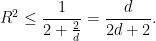
Golden search algorithm – efficient 1D gradient free optimization

Bracketing algorithms for minimizing one dimensional unimodal functions have the form:

• Suppose is an interval containing the minimizer ;
• Pick in and evaluate the function at these points.
• If then choose
• If then choose
• Stop the process when has a length smaller than a given tolerance or a given maximum number of function evaluations is reached.

The simplest algorithm corresponds to choosing which divide the interval into three equal parts. This algorithm can be called trisection algorithm. Below you can see the intervals and intermediary points for a few iterations in the trisection algorithm.

Bracketing intervals and intermediary points for trisection algorithm

Optimizing a 1D function – trisection algorithm

Optimization problems take the classical form

Not all such problems have explicit solution, therefore numerical algorithms may help approximate potential solutions.

Numerical algorithms generally produce a sequence which approximates the minimizer. Information regarding function values and its derivatives are used to generate such an approximation.

The easiest context is one dimensional optimization. The basic intuition regarding optimization algorithms starts by understanding the 1D case. Not all problems are easy to handle for a numerical optimization algorithm. Take a look at the picture below:

photo from Ziv Bar-Joseph

Maximize the circumradius of a unit diameter simplex

Given a simplex in dimension with diameter at most equal to one, what is its largest possible circumradius? The question is well posed, since a ball of diameter will cover all the points (a ball of radius centered at one of the given points).

Consider points in dimension and suppose the origin is the center of the circumscribed ball. Then given two vertices , the circumradius verifies . Therefore, one should maximize the minimal cosine of angles of two such vectors.

An immediate upper bound, which is tight can be obtained from the identity . It can be seen that . Thus the maximal circumradius verifies

This coincides with the case where all angles between different vectors are equal and their cosine is , i.e. the simplex is regular.

Minimal volume of some particular convex sets in the cube

Consider a cube and a convex body contained in it such that the projections of this body on every face of the cube completely covers that face. Prove that the volume of the convex body is at least equal with a third of the volume of the cube.

Graham’s Biggest Little Hexagon

Think of the following problem: What is the largest area of a Hexagon with diameter equal to 1?

As is the case with many questions similar to the one above, called polygonal isoperimetric problems, the first guess is the regular hexagon. For example, the largest area of a Hexagon with fixed perimeter is obtained for the regular hexagon. However, for the initial question, the regular hexagon is not the best one. Graham proved in his paper “The largest small hexagon” that there exists a better competitor and he showed precisely which hexagon is optimal. More details on the history of the problem and more references can be found in Graham’s paper, the Wikipedia page or the Mathworld page.

I recently wanted to use this hexagon in some computations and I was surprised I could not find explicitly the coordinates of such a hexagon. The paper “Isodiametric Problems for Polygons” by Mossinghoff was as close as possible to what I was looking for, although the construction is not explicit. Therefore, below I present a strategy to find what is the optimal hexagon and I will give a precise (although approximate) variant for the coordinates of Graham’s hexagon.

Checking the gradient and Hessian implementation using finite differences

Solving a numerical optimization problem depends not only on the optimization algorithm you use, but also on the fact that you implemented correctly the gradient and, eventually, the Hessian matrix associated to the function you want to optimize. The correct implementation of the partial derivatives is not always a trivial calculus question, where you have an analytic formula for your function and you just need to take care when performing the computations. However, even the best students can make a typing error, put a wrong sign somewhere, miss a factor, etc, and in that case the optimization algorithm simply doesn’t work as expected.

Things get even more complicated when the computation of the gradient (and Hessian) goes through some PDE model, multiplying the places in your code where an error might hide. For example in some parametric shape optimization problem, one has a parametric description of the shape and the gradient of the function to be optimized is obtained by putting in the associated shape derivative formula a perturbation field associated to the variation in the corresponding parameter.

Gradient algorithm with optimal step: Quadratic Case: theory

In a previous post I looked at the theory behind the convergence of the gradient descent algorithm with fixed step for a quadratic function. In this post I will treat a similar topic, namely the gradient descent algorithm with optimal step for the case of a quadratic function. Let us consider again defined by

the classical quadratic function, where is symmetric positive definite and is an arbitrary vector. The gradient descent algorithm with optimal step has the form

where the descent step is chosen such that

is minimal.

Gradient algorithm: Quadratic Case: theory

Everyone who did a little bit of numerical optimization knows the principle gradient descent algorithm. This is the simplest gradient based algorithm: given the current iterate, advance in the opposite direction of the gradient with a given step

It is straightforward to see that if is small enough, and is at least then

This means that there exists a small enough for which .

Are zero-order optimization methods any good?

The short answer is yes, but only when the derivative of gradient of the objective function is not available. To fix the ideas we refer to:

• optimization algorithm: as an iterative process of searching for approximations of a (local/global) minimum of a certain function
• zero-order algorithm: an optimization method which only uses function evaluations in order to decide on the next point in the iterative process.

Therefore, in view of the definitions above, zero-order algorithms want to approximate minimizers of a function using only function evaluations; no further information on derivatives is available. Classical examples are bracketing algorithms and genetic algorithms. The objective here is not to go into detail in any of these algortihms, but to underline one basic limitation which must be taken into account whenever considering these methods.

In a zero-order optimization algorithm any decision regarding the choice of the next iterate can be made only by comparing the values of  at different evaluation points. For example, look at the classical trisection algorithm for minimizing a unimodal function, i.e. a real function defined on which is decreasing on and increasing on :

• given the bracketing choose the points and .
• compare the values and in order to decide on the next bracketing interval:if then

  if then

• stop when the difference is small enough.

One question immediately rises: can such an algorithm reach any desired precision, for example, can it reach the machine precision, i.e. the precision to which computations are done in the software used? To fix the ideas, we’ll suppose that we are in the familiar world of numbers written in double precision, where the machine precision is something like . I will not go into further details regarding this, since people do whole courses on this. Note that Matlab, Octave and Numpy are well known languages in which the default setup uses this machine precision.

More precisely, the real numbers are stored as floating point numbers and only digits are relevant in the computations. When adding two numbers whose ratio is smaller than the result will be . This is due to the fact that adding the numbers would require us to shift the decimal point to the same position. However, since the ratio is smaller than , when shifting the decimal point to the same position, the resulting number will contain zeros on the first or more significant digits in . Therefore the addition will not change any significant digits in .

This issue related to computations done in floating point precision makes the question of comparing and in the algorithm above pointless when and are close to the minimum. In order to identify the source of the potential problem let us write the Taylor expansion of the function around the minimum . First, note that at the minimum, which leaves us with

where denotes higher order terms. You may note that neglecting higher order terms shows that the function looks like a quadratic function near the optimum. This is a good thing to keep in mind and students should not hold any grudge for professors who illustrate the behavior of optimization algorithms on quadratic functions. As it turns out, any good algorithm needs to behave well for quadratic functions, since every function, near a minimum is eventually quadratic.

Coming back to our previous paragraph, it turns out that the computer won’t be able to tell the difference between and if

where is the machine precision. Therefore, if

the machine won’t tell the difference between and . Since the second factor in the above expression is well defined and positive in most cases, it turns out that we will not be able to decide if we are closer than to the solution based only on the values of the function .

Therefore, when using a zero-order algorithms for a function with you cannot decide based only on the function values if you are closer to the optimum than the square root of the machine precision . This is quite a limitation, and in practice it should save lots of pointless function evaluations.

When using derivatives or gradients there is no such problem, since we can decide if we are close enough to by comparing the derivative to zero, and this comparison is valid up to the precision to which we can compute .

In conclusion, use zero-order methods only if gradient based methods are out of reach. Zero-order methods are not-only slowly convergent, but may also be unable to achieve the expected precision in the end.

Optimality conditions – equality constraints

Everyone knows that local minima and maxima of a function are critical points, i.e. points where the gradient is equal to zero. This is what we call an optimality condition, a condition verified by every solution of a minimization or maximization problem.

The situation changes when dealing with constraints. Consider a simple example, like and note that the gradient of the objective function is not zero at the optimal solution . The idea is that one needs to take into account the constraint when writing optimality conditions in this case. This leads us to consider the theory of Lagrange multipliers. Every student finds this concept a bit difficult when seen for the first time.

Since a picture is worth 1000 words, let me share with you two pictures 🙂  Consider the minimization of under the constraint . The first photo below shows the gradients of the function and the constraint at the optimal solution approximated numerically. One striking property becomes obvious: the gradient of the function aligns with the gradient of the constraint. In order to see why this is necessary, let us look at another point in the constraint set where the two gradients are not aligned, shown in the second picture.

It becomes obvious that if the two gradients are not aligned, then there exists a component of which is tangent to the constraint set. Therefore, going along this direction, in its opposite sense it is possible to further decrease the value of the function , while still following the constraint set. Therefore, when the two gradients are not aligned we are not at a minimum (the same type of argument works for maximizing problems).

Of course, this geometric argument is not the whole picture, but it gives an important insight, which directly implies the theory of Lagrange multipliers: at the optimum, the gradient should be orthogonal to the tangent space to the constraint set, and this orthogonal, under some regularity assumptions, is generated by the gradients of the constraints themselves, giving the famous relation

Now, once we understood the intuition behind this, it remains to see under which conditions there exists a tangent space to the constraints set, and see rigorously why the above relation holds. But all this is left for some future post.

Gradient Descent converging to a Saddle Point

Gradient descent (GD) algorithms search numerically for minimizers of functions . Once an initialization is chosen the algorithm is defined by

where is a descent step, often found using a particular line-search procedure. It is widely known that GD algorithms converge to critical points under very mild hypotheses on the function and on the line-search procedure. Moreover, GD algorithms almost always converge to local minimizers (convergence to the global minimizer is hard to guarantee, except in the convex case).

However, the “almost always” part from the above sentence is in itself interesting. It turns out that the choice of the initialization may lead the algorithm to get stuck in a Saddle Point, i.e. a critical point where the Hessian matrix has both positive and negative eigenvalues. The way to imagine such examples is to note that at such a Saddle Point there are directions for which is minimized and directions for which is maximized. If the gradient only contains information in the direction where is minimized, the algorithm will stop there. However, the set of initializations for which GD will get stuck in a Saddle Point is very small and considering slightly perturbed initializations might solve the problem.

To better illustrate this phenomenon, let’s look at a two dimensional example:

It can be seen immediately that this function has critical points at and that is a saddle point, while the other two are local minima. A graph of this function around the origin is shown below

Note that looking only along the line the saddle point is a minimizer. Therefore, choosing an initialization on this line will make the GD algorithm be stuck in the Saddle Point . Below you can see an example for the initialization , and the trajectory of the GD algorithm is illustrated. Considering only a slight perturbation allows the GD algorithm to escape the saddle point and to converge to a local minimizer.

 

One simple way to prevent GD algorithms being stuck in a saddle point is to consider randomized initializations so that you avoid any bias you might have regarding the objective function.

Computing the Shape Derivative of the Wentzell Problem

Computing shape derivatives is a nice thing to know if you do numerical shape optimization. When you want to minimize a quantity depending on a shape in a more or less direct way, you should be able to differentiate it so that gradient algorithms could be applied. Computing shape derivatives is not that easy, but below there is a method which is not that hard once you practice some simple examples. For some bibliography on the subject I present you the following:

• Jean CEA, Conception optimale ou identification de formes, calcul rapide de la dérivée directionnelle de la fonction coût: this is in French, but it presents the method nicely.
• Chicco-Ruiz, Morin, Pauletti, The shape derivative of the Gauss curvature. This is not an original source of the classical results, but it contains a very nice summary of the basic notions of shape derivatives.
• Delfour, Zolesio, Shapes and Geometries
• Henrot, Pierre, Shape Variation and Optimization
• Gregoire Allaire, see his the shape optimization course on his homepage

We start directly with a complicated example, containing some complex boundary terms. The Wentzell eigenvalue problem is given by the following:

It is not hard to see that the associated variational formulation is given by

Lagrangians – derivation under constraints

In this post I will describe a formal technique which can help in finding derivatives of functions under certain constraints. In order to see what I mean, take the following two examples:

1. If you differentiate the function with respect to , you get zero, obviously.

2. If you differentiate the function under the constraint that (supposing that ) then it is not hard to see that and the derivative will be .

This shows that adding certain constraints will change the derivative and when dealing with more sophisticated constraints, like PDE or differential equations, things get less clear.

The question of the existence of derivatives with respect to some variables, when dealing with constraints, is usually dealt with by using the implicit function theorem: this basically says that if some variables are linked by some smooth equations and that you can locally invert the dependence, then you can infer differentiability.

The method presented below skips this step and goes directly for the computation of the derivative. This is a common used technique in control theory or shape optimization, where computing derivatives is essential in numerical simulations. I will come back to derivatives linked to shape optimization in some further posts. For now, let’s see how one can use the Lagrangian method for computing derivatives in some simple cases.

Example 1. Let’s compute the derivative of under the constraint . In order to do this we introduce a Lagrangian, which has the following form

Example of optimization under constraints – using Lagrange multipliers

Consider the functional defined by

and the set defined by .

1. Prove that admits a minimizer on and find it.
2. Let be the set . Does admit minimizers on ? If yes determine all points in which the maximum is attained.

Proof: This is a problem which illustrates well concepts related to optimality conditions for constrained problems. It is possible to solve these problems by two methods: one using only basic ideas and a second one using results from optimization theory. One can also see by examining the basic method how to recover naturally the optimality condition given by the Lagrange multipliers.

Optimizing a quadratic functional under affine constraints

Consider the quadratic functional defined by

for a real matrix which is symmetric positive definite and a vector . Consider also the application defined by where is a real matrix and . Furthermore suppose that and that is of maximal rank. The objective is to study the following optimization problem under equality constraints:

where is defined by .

1. Show that has a unique minimizer on .
2. Prove that if is the minimizer of on then there exists a unique vector such that solves the linear system

   

3. Show that the matrix of the above system is invertible.

Project Euler 607

If you like solving Project Euler problems you should try Problem number 607. It’s not very hard, as it can be reduced to a small optimization problem. The idea is to find a path which minimizes time, knowing that certain regions correspond to different speeds. A precise statement of the result can be found on the official page. Here’s an image of the path which realizes the shortest time:

 

Project Euler tips

A few years back I started working on Project Euler problems mainly because it was fun from a mathematical point of view, but also to improve my programming skills. After solving about 120 problems I seem to have hit a wall, because the numbers involved in some of the problems were just too big for my simple brute-force algorithms.

Recently, I decided to try and see if I can do some more of these problems. I cannot say that I’ve acquired some new techniques between 2012-2016 concerning the mathematics involved in these problems. My research topics are usually quite different and my day to day programming routines are more about constructing new stuff which works fast enough than optimizing actual code. Nevertheless, I have some experience coding in Matlab, and I realized that nested loops are to be avoided. Vectorizing the code can speed up things 100 fold.

So the point of Project Euler tasks is making things go well for large numbers. Normally all problems are tested and should run within a minute on a regular machine. This brings us to choosing the right algorithms, the right simplifications and finding the complexity of the algorithms involved.

IMC 2016 – Day 2 – Problem 7

Problem 7. Today, Ivan the Confessor prefers continuous functions satisfying for all . Fin the minimum of over all preferred functions.

SIAM 100 digit challenge no 4 – Matlab solution

In 2002 the SIAM News magazine published a list of problems in numerical analysis. The answer to each of the problems should be given with an accuracy of at least digits. And so there came the Hundred-Dollar, Hundred-Digit Challenge. I present below my attempt to solving the th problem in this series, as it deals to finding the global minimum of a highly oscillating function. I confess that my approach is rather simplistic, but solves the problem. First let’s state the problem below:

Problem 4. What is the global minimum of the function