Optimizing a 1D function – trisection algorithm

Optimization problems take the classical form

Not all such problems have explicit solution, therefore numerical algorithms may help approximate potential solutions.

Numerical algorithms generally produce a sequence which approximates the minimizer. Information regarding function values and its derivatives are used to generate such an approximation.

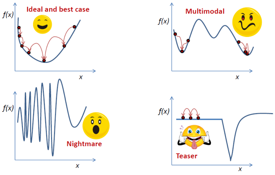
The easiest context is one dimensional optimization. The basic intuition regarding optimization algorithms starts by understanding the 1D case. Not all problems are easy to handle for a numerical optimization algorithm. Take a look at the picture below:

photo from Ziv Bar-Joseph

For simplicity, let us assume that is a unimodal function: there exists such that is decreasing on and increasing on .

Furthermore, suppose that we can only compute values (not derivatives). This is true for various practical applications:

• the function value might come from an experiment.
• the value might be related to a solution of a mathematical model which is hard to differentiate
• the function may simply come from a black box device. We have a way to obtain values, but not derivatives.

For such a function (assuming it is unimodal, it has a unique local minimum) it is possible to devise a bracketing algorithm for finding the minimizer . Take a moment to think how many function evaluations for points in are needed to find a tighter enclosure for ?

A quick inspection shows that one function evaluation does not give enough information. Suppose that

Then:

• if the minimizer cannot lie in . Therefore is a guaranteed inclusion for .
• if the minimizer cannot lie in . Therefore is a guaranteed inclusion for .

This gives rise to a straightforward iterative algorithm. All we need is a systematic way of choosing in and iterate such that the length of the bracketing interval converges to .

The simplest idea is to use the trisection algorithm where divide into three equal parts. At every iteration the length of the bracketing interval is multipled by , therefore a satisfying error will be attained after a reasonable number of iterations. A simple Python implementation is given below:

def Trisection(fun,A,B,tol=1e-6,ubFeval=10):
    nfeval = 0
    lbhist = []
    ubhist = []
    x1hist = []
    x2hist = []
    lb = A
    ub = B
    lbhist.append(lb)
    ubhist.append(ub)
    while ub-lb>tol:
        x1 = 2/3*lb+1/3*ub
        x2 = 1/3*lb+2/3*ub
        v1 = fun(x1)
        nfeval = nfeval+1
        if nfeval>=ubFeval:
            break
        v2 = fun(x2)
        nfeval = nfeval+1
        if v1<=v2:
            ub=x2
        else:
            lb=x1
        x1hist.append(x1)
        x2hist.append(x2)
        lbhist.append(lb)
        ubhist.append(ub)
        if nfeval>=ubFeval:
            break
    return np.array(lbhist),np.array(ubhist),np.array(x1hist),np.array(x2hist),nfeval

Since the error estimate , equal to the distance from to the midpoint of , for example, verifies an inequality of the form

we say that this algorithm converges linearly.

One drawback of trisection algorithm is that two function evaluations are made at every iteration. This can be improved with a slight modification which we’ll cover soon.